Is Lm Curve Money Supply Increase

Chapter 22 IS-LM in Action

Chapter Objectives

Past the cease of this chapter, students should be able to:

Explain what causes the liquidity preference–money (LM) curve to shift and why.
Explain what causes the investment-savings (IS) curve to shift and why.
Explain the difference between monetary and fiscal stimulus in the brusk term and why the deviation is important.
Explain what happens when the IS-LM model is used to tackle the long term by taking changes in the price level into business relationship.
Describe the aggregate demand bend and explain what causes it to shift.

22.1 Shifting Curves: Causes and Effects

Learning Objective

What causes the LM and IS curves to shift and why?

Policymakers can use the IS-LM model developed in Chapter 21 "IS-LM"to help them determine between 2 major types of policy responses, fiscal (or government expenditure and revenue enhancement) or monetary (interest rates and money). As you probably noticed when playing around with the IS and LM curves at the end of the previous affiliate, their relative positions matter quite a fleck for involvement rates and aggregate output. Time to investigate this matter further.

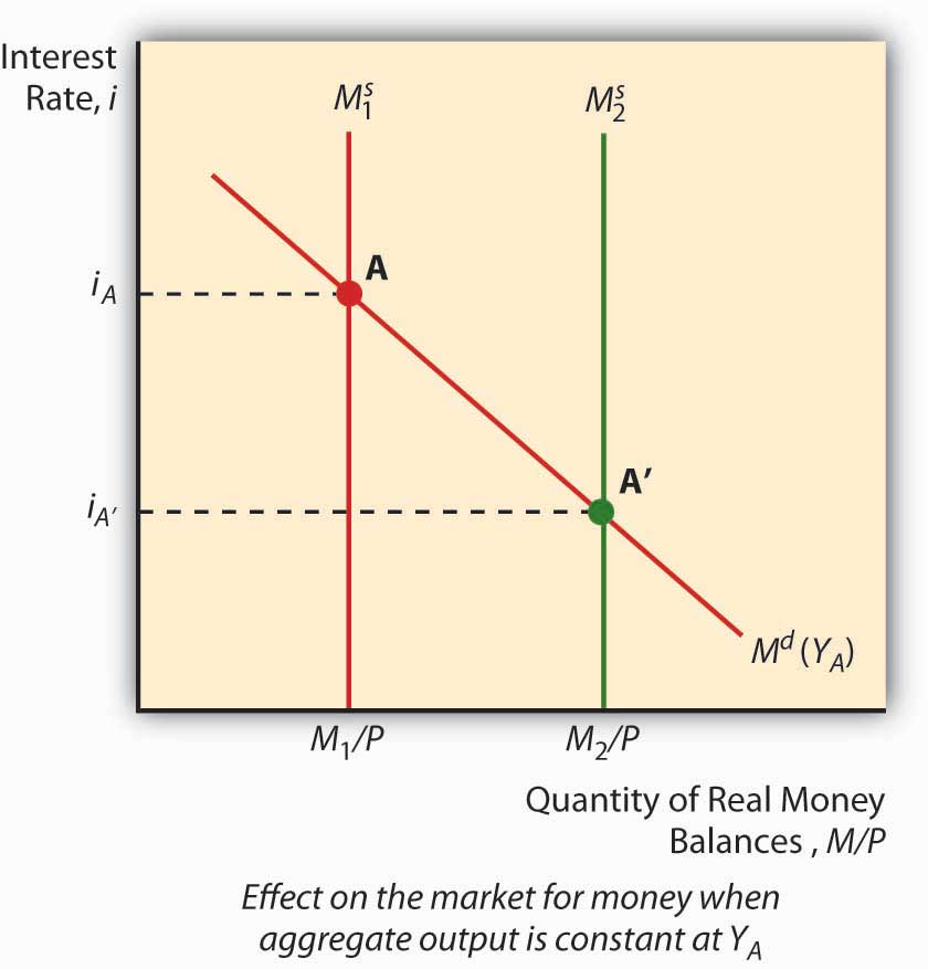
The LM curve, the equilibrium points in the market place for coin, shifts for 2 reasons: changes in coin demand and changes in the money supply. If the coin supply increases (decreases), ceteris paribus, the interest charge per unit is lower (college) at each level of Y, or in other words, the LM curve shifts correct (left). That is because at any given level of output Y, more money (less money) means a lower (college) interest rate. (Call up, the price level doesn't change in this model.) To see this, look at Figure 22.1 "Effect of money on interest rates when output is constant".

Figure 22.1 Effect of money on interest rates when output is constant

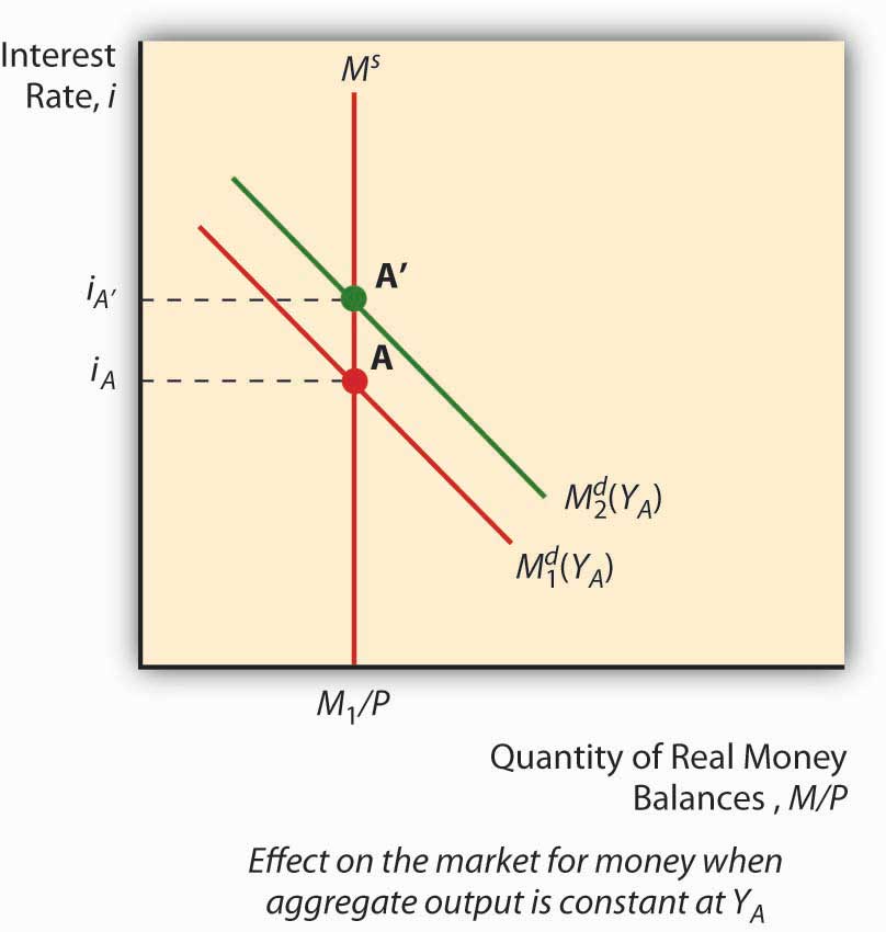
An autonomous change in coin demand (that is, a change non related to the cost level, aggregate output, or i) will also affect the LM curve. Say that stocks get riskier or the transaction costs of trading bonds increases. The theory of nugget demand tells us that the demand for money will increase (shift correct), thus increasing i. Involvement rates could also decrease if money need shifted left because stock returns increased or bonds became less risky. To run into this, examine Figure 22.2 "Effect of an autonomous change in money demand when output is abiding". An increment in autonomous coin need will shift the LM bend left, with higher involvement rates at each Y; a decrease volition shift it right, with lower interest rates at each Y.

Figure 22.two Effect of an autonomous change in money demand when output is constant

The IS curve, by contrast, shifts whenever an democratic (unrelated to Y or i) change occurs in C, I, M, T, or NX. Following the word of Keynesian cross diagrams in Chapter 21 "IS-LM", when C, I, G, or NX increases (decreases), the IS bend shifts right (left). When T increases (decreases), all else constant, the IS curve shifts left (right) because taxes effectively decrease consumption. Again, these are changes that are non related to output or interest rates, which merely indicate movements forth the IS curve. The discovery of new caches of natural resources (which will increase I), changes in consumer preferences (at domicile or away, which will affect NX), and numerous other "shocks," positive and negative, will change output at each interest rate, or in other words shift the entire IS curve.

We can now see how regime policies can affect output. Equally noted higher up, in the short run, an increase in the money supply volition shift the LM curve to the right, thereby lowering interest rates and increasing output. Decreasing the MS would have precisely the opposite effect. Financial stimulus, that is, decreasing taxes (T) or increasing government expenditures (G), will besides increment output but, unlike monetary stimulus (increasing MS), will increase the interest rate. That is because it works by shifting the IS curve upward rather than shifting the LM curve. Of grade, if T increases, the IS curve will shift left, decreasing interest rates but also aggregate output. This is part of the reason why people get hot under the collar nearly taxes.See, for example, www.nypost.com/p/news/opinion/opedcolumnists /soaking_the_rich_AW6hrJYHjtRd0Jgai5Fx1O (Of course, individual considerations are paramount!)www.politicususa.com/en/polls-taxes-deficit. Notation that the people supporting taxation increases typically support raising other people's taxes: "The poll also found wide support for increasing taxes, as 67% said the more than loftier earners income should be field of study to being taxed for Social Security, and 66% support raising taxes on incomes over $250,000, and 62% back up endmost corporate taxation loopholes."

Stop and Think Box

During financial panics, economical agents complain of loftier involvement rates and declining economic output. Utilise the IS-LM model to describe why panics have those furnishings.

The LM bend will shift left during panics, raising involvement rates and decreasing output, because demand for money increases as economic agents scramble to get liquid in the face of the declining and volatile prices of other assets, specially fiscal securities with positive default risk.

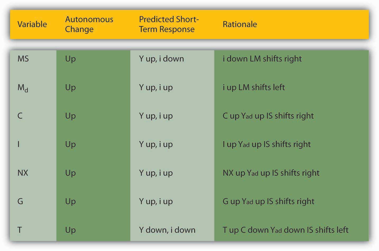
Effigy 22.3 "Predicted effects of changes in major macroeconomic variables"summarizes.

Figure 22.3 Predicted effects of changes in major macroeconomic variables

Stop and Recollect Box

Describe Hamilton'southward Police (née Bagehot'south Police) in terms of the IS-LM model. Hint: Hamilton and Bagehot argued that, during a financial panic, the lender of last resort needs to increase the money supply by lending to all comers who present what would be considered acceptable collateral in normal times.

During financial panics, the LM bend shifts left as people flee risky assets for money, thereby inducing the interest rate to climb and output to fall. Hamilton and Bagehot argued that budgetary regime should respond by nipping the problem in the bud, and then to speak, by increasing MS directly, shifting the LM curve back to somewhere most its pre-panic position.

Primal Takeaways

The LM curve shifts right (left) when the money supply (real money balances) increases (decreases).
It besides shifts left (right) when money need increases (decreases).
The easiest way to meet this is to beginning imagine a graph where money demand is fixed and the money supply increases (shifts correct), leading to a lower involvement rate, and vice versa.
So imagine a fixed MS and a shift upwards in money demand, leading to a higher interest charge per unit, and vice versa.
The IS bend shifts right (left) when C, I, G, or NX increase (decrease) or T decreases (increases).
This relates directly to the Keynesian cross diagrams and the equation Y = C + I + K + NX discussed in Chapter 21 "IS-LM", and also to the analysis of taxes as a decrease in consumption expenditure C.

22.2 Implications for Budgetary Policy

Learning Objectives

In the short term, what is the difference between monetary and fiscal stimulus and why is it important?
What happens when the IS-LM model is used to tackle the long term by taking changes in the price level into business relationship?

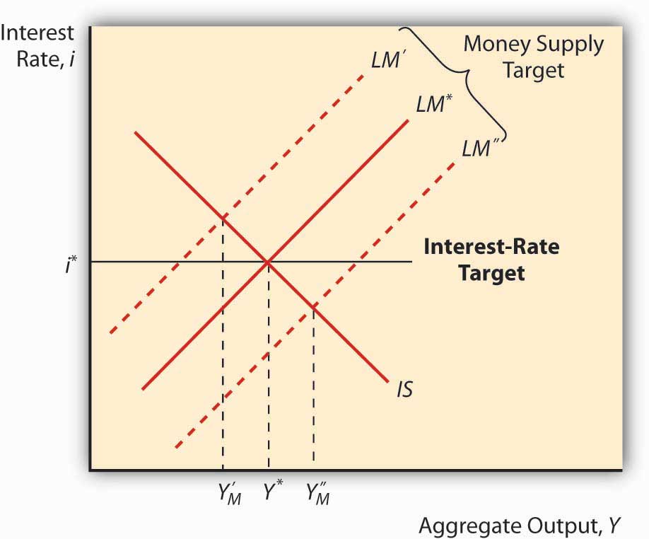
The IS-LM model has a major implication for monetary policy: when the IS curve is unstable, a coin supply target will lead to greater output stability, and when the LM curve is unstable, an involvement charge per unit target volition produce greater macro stability. To come across this, await at Figure 22.four "Effect of IS curve instability" and Figure 22.five "Upshot of LM curve instability". Note that when LM is stock-still and IS moves left and correct, an interest rate target will cause Y to vary more than a money supply target volition. Notation too that when IS is fixed and LM moves left and right, an involvement rate target keeps Y stable but a money supply target (shifts in the LM curve) will cause Y to swing wildly. This helps to explain why many fundamental banks abased coin supply targeting in favor of interest charge per unit targeting in the 1970s and 1980s, a period when autonomous shocks to LM were pervasive due to financial innovation, deregulation, and loophole mining. An important implication of this is that primal banks might detect it prudent to shift back to targeting monetary aggregates if the IS bend ever again becomes more unstable than the LM curve.

Figure 22.iv Effect of IS curve instability

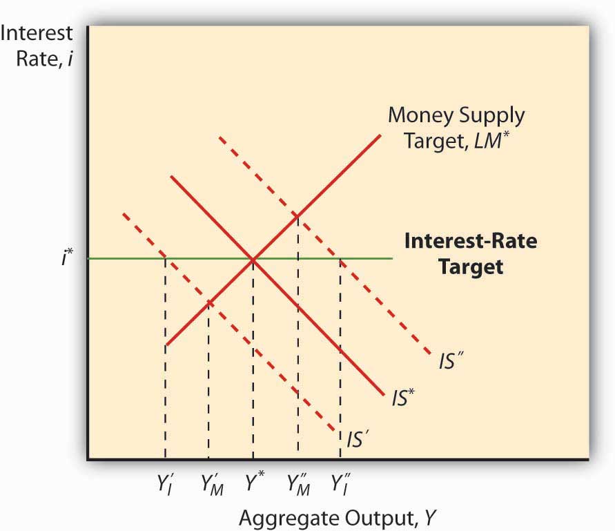
Figure 22.5 Effect of LM bend instability

As noted in Chapter 21 "IS-LM", the policy power of the IS-LM is severely limited by its short-run assumption that the price level doesn't change. Attempts to tweak the IS-LM model to adapt price level changes led to the creation of an entirely new model called aggregate demand and supply. The key is the add-on of a new concept, called the natural charge per unit level of outputThe charge per unit of output at which the price level has no tendency to rise or fall. , Y_nrl, the rate of output at which the toll level is stable in the long run. When actual output (Y*) is below the natural rate, prices will fall; when it is to a higher place the natural charge per unit, prices will rise.

The IS curve is stated in real terms because it represents equilibrium in the goods marketplace, the real role of the economy. Changes in the price level therefore do not touch on C, I, G, T, or NX or the IS bend. The LM curve, however, is affected by changes in the price level, shifting to the left when prices rise and to the right when they autumn. This is considering, holding the nominal MS constant, rise prices subtract real money balances, which we know shifts the LM bend to the left.

So suppose an economic system is in equilibrium at Y_nrl, when some budgetary stimulus in the grade of an increased MS shifts the LM bend to the correct. As noted above, in the short term, interest rates will come down and output will increase. But because Y* is greater than Y_nrl, prices volition ascent, shifting the LM bend dorsum to where it started, give or take. So output and the interest rate are the same but prices are higher. Economists call this long-run monetary neutrality.

Fiscal stimulus, as we saw above, shifts the IS curve to the correct, increasing output just also the interest rate. Because Y* is greater than Y_nrl, prices will ascension and the LM curve will shift left, reducing output, increasing the interest rate higher still, and raising the price level! You just can't win in the long run, in the sense that policymakers cannot make Y* exceed Y_nrl . Rendering policymakers impotent did not win the IS-LM model many friends, so researchers began to develop a new model that relates the price level to amass output.

Stop and Call up Box

Nether the gold standard (GS), money flows in and out of countries automatically, in response to changes in the price of international bills of exchange. From the standpoint of the IS-LM model, what is the trouble with that aspect of the GS?

As noted above, decreases in MS lead to a leftward shift of the LM curve, leading to higher involvement rates and lower output. Higher involvement rates, in turn, could pb to a financial panic or a decrease in C or I, causing a shift left in the IS curve, farther reducing output simply relieving some of the pressure on i. (Note that NX would not exist affected under the GS because the commutation rate was fixed, moving just within very tight bands, so a higher i would not cause the domestic currency to strengthen.)

Key Takeaways

Monetary stimulus, that is, increasing the money supply, causes the LM bend to shift right, resulting in college output and lower interest rates.
Fiscal stimulus, that is, increasing government spending and/or decreasing taxes, shifts the IS curve to the right, raising interest rates while increasing output.
The higher interest rates are problematic because they tin can oversupply out C, I, and NX, moving the IS bend left and reducing output.
The IS-LM model predicts that, in the long run, policymakers are impotent.
Policymakers can enhance the price level merely they can't become Y* permanently above Y_nrl or the natural rate level of output.
That is because whenever Y* exceeds Y_nrl, prices rise, shifting the LM bend to the left past reducing real money balances (which happens when in that location is a higher toll level coupled with an unchanged MS).
That, in turn, eradicates any gains from budgetary or financial stimulus.

22.3 Aggregate Demand Bend

Learning Objective

What is the amass demand (AD) curve and what causes it to shift?

Imagine a fixed IS curve and an LM curve shifting difficult left due to increases in the price level, as in Effigy 22.6 "Deriving the amass demand bend". As prices increase, Y falls and i rises. Now plot that upshot on a new graph, where aggregate output Y remains on the horizontal axis but the vertical axis is replaced past the toll level P. The resulting curve, chosen the aggregate demand (Advert) bend, will slope downwardly, as beneath. The Advertizing bend is a very powerful tool considering information technology indicates the points at which equilibrium is achieved in the markets for goods and money at a given price level. It slopes down because a high toll level, ceteris paribus, means a small real money supply, high interest rates, and a low level of output, while a low toll level, all else constant, is consequent with a larger real coin supply, low interest rates, and kickin' output.

Effigy 22.half dozen Deriving the aggregate demand curve

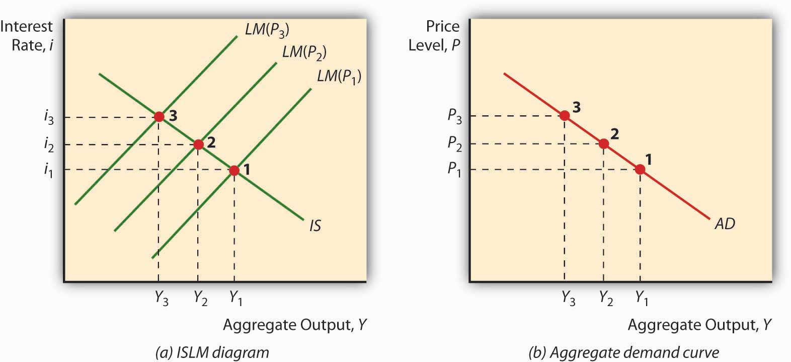
Because the AD curve is substantially just another style of stating the IS-LM model, anything that would modify the IS or LM curves will besides shift the AD curve. More than specifically, the AD curve shifts in the same direction every bit the IS curve, and then it shifts right (left) with autonomous increases (decreases) in C, I, G, and NX and decreases (increases) in T. The AD curve as well shifts in the same direction as the LM bend. So if MS increases (decreases), it shifts right (left), and if 1000_d increases (decreases) information technology shifts left (right), as in Figure 22.three "Predicted effects of changes in major macroeconomic variables".

Key Takeaways

The aggregate demand curve is a downward sloping curve plotted on a graph with Y on the horizontal axis and the toll level on the vertical axis.
The AD curve represents IS-LM equilibrium points, that is, equilibrium in the market for both appurtenances and coin.
It slopes downwards because, as the price level increases, the LM curve shifts left equally real money balances fall.
AD shifts in the same management as the IS or LM curves, and so anything that shifts those curves shifts Advertizing in precisely the same management and for the aforementioned reasons.

22.four Suggested Reading

Dimand, Robert, Edward Nelson, Robert Lucas, Mauro Boianovsky, David Colander, Warren Young, et al. The IS-LM Model: Its Ascent, Fall, and Strange Persistence. Raleigh, NC: Duke University Press, 2005.

Young, Warren, and Ben-Zion Zilbefarb. IS-LM and Mod Macroeconomics. New York: Springer, 2001.